ERP常规处理代码解析
posted on 04 Mar 2019 under category EEG
前面两篇文章主要解决的是ERP数据预处理的问题,预处理完后就要开始根据实验设计的需求进行各种分析了,其中最经典的两个指标就是波幅和潜伏期。那么,在这篇文章中,我们要解决的问题就是如何用代码来计算ERP经典成分的波幅和潜伏期并作图。
下面是整个处理的完整代码:
clear all; clc;

%% part1: compute group-level ERP

Subj = [1:10]; %% subject numbers
for i = 1:length(Subj)
    setname = strcat(num2str(i),'_LH.set'); %% filename of set file
    setpath = 'D:\day23\day23\Example_data\'; %% filepath of set files (need to be changed)
    EEG = pop_loadset('filename',setname,'filepath',setpath); %% load the data
    EEG = eeg_checkset( EEG );
    EEG_avg(i,:,:) = squeeze(mean(EEG.data,3)); %% single-subject ERPs; EEG_avg dimension: subj*channel*time
end
save('Group_level_ERP.mat','EEG_avg');  %% save the data of subjects

%% part2: plot group-level ERP

Cz=13; % select the channel to plot (display maximum response)
figure;
mean_data=squeeze(mean(EEG_avg(:,Cz,:),1)); %% select the data at Cz, average across subjects, mean_data: 1*3000
plot(EEG.times, mean_data,'k','linewidth', 1.5); %% plot the waveforms
set(gca,'YDir','reverse'); %% reverse the direction of Y axis
axis([-500 1000 -15 10]);  %% define the region to display
title('Group-level at Cz','fontsize',16); %% specify the figure name
xlabel('Latency (ms)','fontsize',16); %% name of X axis
ylabel('Amplitude (uV)','fontsize',16);  %% name of Y axis

%% part3: plot the scalp maps at dominant peaks

N2_peak = 207; P2_peak=374; %% dominant peaks on waveforms
N2_interval = find((EEG.times>=197)&(EEG.times<=217)); %% define the N2 intervals [peak-10 peak+10]
P2_interval = find((EEG.times>=364)&(EEG.times<=384)); %% define the P2 intervals [peak-10 peak+10]

N2_amplitude = squeeze(mean(EEG_avg(:,:,N2_interval),3));  %% N2 amplitude for each subject and each channel
P2_amplitude = squeeze(mean(EEG_avg(:,:,P2_interval),3));   %% P2 amplitude for each subject and each channel

Central = [13 14];
N2_measures = squeeze(mean(mean(EEG_avg(:,Central,N2_interval),2),3));  %% N2 amplitude for each subject  (for statistics)
P2_measures = squeeze(mean(mean(EEG_avg(:,Central,P2_interval),2),3));   %% P2 amplitude for each subject  (for statistics)

figure;
subplot(121); topoplot(mean(N2_amplitude),EEG.chanlocs,'maplimits',[-15 15]); title('N2 Amplitude','fontsize',16); %% N2 scalp map (group-level)
subplot(122); topoplot(mean(P2_amplitude),EEG.chanlocs,'maplimits',[-15 15]); title('P2 Amplitude','fontsize',16); %% P2 scalp map (group-level)

%% part4: series of scalp mps

time_interval = [0:100:500]; %% specify the time intervals to display (to be changed)
figure;
for i = 1:length(time_interval)
    latency_range = [time_interval(i) time_interval(i)+100]; %% lower and upper limits
    latency_idx = find((EEG.times>=latency_range(1))&(EEG.times<=latency_range(2))); %% interval of the specific regions
    Amplitude = squeeze(mean(mean(EEG_avg(:,:,latency_idx),1),3)); %% 1*channel (averaged across subjects and interval)
    subplot(2,3,i);
    topoplot(Amplitude,EEG.chanlocs,'maplimits',[-10 10]); %% topoplot(Amplitude,EEG.chanlocs);
    setname=strcat(num2str(latency_range(1)),'--',num2str(latency_range(2)),'ms'); %% specify the name of subplots
    title(setname,'fontsize',16); %% display the names of subplots
end
就如注释中标注的一致,这段代码可以分为4个部分,分别是计算组水平的ERP、画出ERP的图形、画出峰值处的地形图以及画出时间系列的地形图。下面就分四个部分解释代码:
计算组水平的ERP
%% part1: compute group-level ERP

Subj = [1:10]; %% subject numbers
for i = 1:length(Subj)
    setname = strcat(num2str(i),'_LH.set'); %% filename of set file
    setpath = 'D:\day23\day23\Example_data\'; %% filepath of set files (need to be changed)
    EEG = pop_loadset('filename',setname,'filepath',setpath); %% load the data
    EEG = eeg_checkset( EEG );
    EEG_avg(i,:,:) = squeeze(mean(EEG.data,3)); %% single-subject ERPs; EEG_avg dimension: subj*channel*time
end
save('Group_level_ERP.mat','EEG_avg');  %% save the data of subjects
这段代码的基本功能是导入被试的数据,将一个个被试的数据汇聚成一组数据。这里需要注意的是导入的数据是经过我们之前预处理后的数据。代码中的前面几行在上一篇文章中已经做过解释了,这里就只解释一行代码:
EEG_avg(i,:,:) = squeeze(mean(EEG.data,3)); %% single-subject ERPs; EEG_avg dimension: subj*channel*time
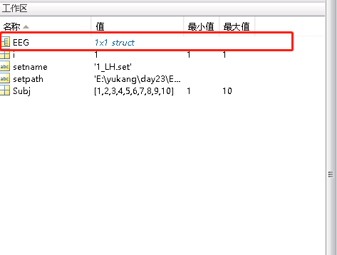
导入被试的数据之后,我们可以在matlab的工作区上看到:
当你鼠标双击EEG之后,会出现如下界面:
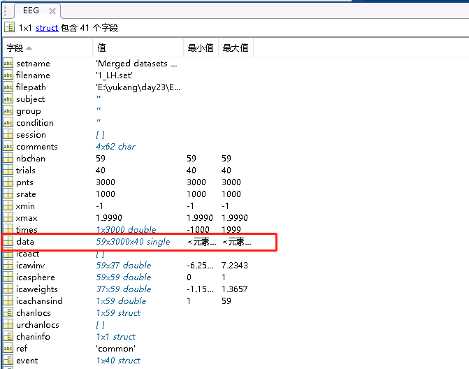
可以发现,data的数据结构是三维数据,三个维度分别是电极、时间点和trial的数量。代码中 mean(EEG.data,3) 的意思就是将data的第三个维度(即trial)给平均。而函数 squeeze 的功能就是降维,即将data原有的三维数据给降为二维数据(电极时间点),然后再将这二位数据加上被试维度组成一个新的三维数据赋值给变量 EEG_avg,这样现在的数据的维度就变成了被试电极点*时间点。然后,这段代码的最后一行是把数据给保存起来。
画组水平的ERP图
%% part2: plot group-level ERP

Cz=13; % select the channel to plot (display maximum response)
figure;
mean_data=squeeze(mean(EEG_avg(:,Cz,:),1)); %% select the data at Cz, average across subjects, mean_data: 1*3000
plot(EEG.times, mean_data,'k','linewidth', 1.5); %% plot the waveforms
set(gca,'YDir','reverse'); %% reverse the direction of Y axis
axis([-500 1000 -15 10]);  %% define the region to display
title('Group-level at Cz','fontsize',16); %% specify the figure name
xlabel('Latency (ms)','fontsize',16); %% name of X axis
ylabel('Amplitude (uV)','fontsize',16);  %% name of Y axis
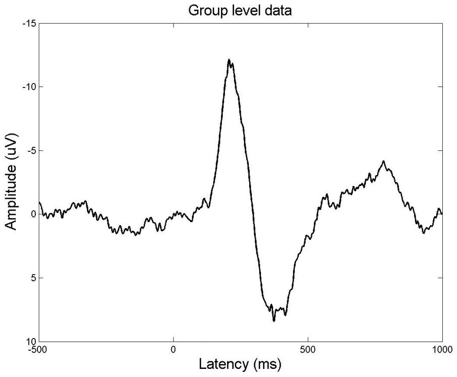
这一段代码的功能是画ERP图,代码中的第一行是选择电极点(根据自己要分析的成分对应的电极进行改动)。后面的 figure 是一个生成画布命令。squeeze(mean(EEG_avg(:,Cz,:),1)) 的功能就是将变量EEG_avg的第一个维度(被试)给平均,然后再降维,最后将值赋给变量mean_data。这样的话现在的变量 mean_data 就变成了一维数据(时间点)。plot(EEG.times,mean_data,'k','linewith',1.5)的功能就是画图,图形包括x轴和y轴两个维度的数据,其中EEG_times是x轴数据(时间维度),而mean_data就是y轴数据(波幅),后面的就是设置图形中线条的颜色,线宽等具体参数。set(gca,'YDir','reverse') 的功能就是将y轴的正负方向给颠倒(在ERP作图中有一个不成文的规定,就是负轴朝上,正轴朝下)。axis([-500 1000 -15 10]) 就是设置横轴和纵轴的标度范围。title('Group-level at Cz','fontsize',16) 就是设置标题及其字体的大小,最后两行分别是设置横轴和纵轴的名称及其字体大小。这个部分跑完之后会自动生成如下图形:
画峰值处的地形图
%% part3: plot the scalp maps at dominant peaks

N2_peak = 207; P2_peak=374; %% dominant peaks on waveforms
N2_interval = find((EEG.times>=197)&(EEG.times<=217)); %% define the N2 intervals [peak-10 peak+10]
P2_interval = find((EEG.times>=364)&(EEG.times<=384)); %% define the P2 intervals [peak-10 peak+10]

N2_amplitude = squeeze(mean(EEG_avg(:,:,N2_interval),3));  %% N2 amplitude for each subject and each channel
P2_amplitude = squeeze(mean(EEG_avg(:,:,P2_interval),3));   %% P2 amplitude for each subject and each channel

Central = [13 14];
N2_measures = squeeze(mean(mean(EEG_avg(:,Central,N2_interval),2),3));  %% N2 amplitude for each subject  (for statistics)
P2_measures = squeeze(mean(mean(EEG_avg(:,Central,P2_interval),2),3));   %% P2 amplitude for each subject  (for statistics)

figure;
subplot(121); topoplot(mean(N2_amplitude),EEG.chanlocs,'maplimits',[-15 15]); title('N2 Amplitude','fontsize',16); %% N2 scalp map (group-level)
subplot(122); topoplot(mean(P2_amplitude),EEG.chanlocs,'maplimits',[-15 15]); title('P2 Amplitude','fontsize',16); %% P2 scalp map (group-level)
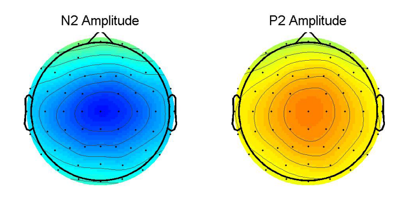
第一行代码的作用是定位峰值的时间点,其中N2成分的峰值在207毫秒处,P2成分的峰值在374毫秒处(这个要在上一个生成的图形里面找峰值,在图形的画布菜单栏中有一个游标,游标指定线条上的某个位置就会自动的显示出该位置的坐标参数)。下面两行代码的 find 函数的功能是寻找N2和P2两个成分对应的索引,计算的方法是取峰值处前后各10毫秒的均值作为峰值的值。变量N2_amplitude和P2_amplitude是作为后续统计使用的。最后两行代码是用来画拓扑图的,subplot函数是用来画子画布的,括号中的数字121的含义是画两个图,两图的排列方式是按照1排2列的方式排列,然后当前的图形是第一个图,同理122是当前图形中的第二个图。topoplot函数的功能是画地形图,函数中包含的参数有ERP波幅值、电极点信息和能量分布的范围。这段代码执行完后,会自动生成如下图形:
画时间系列的地形图
%% part4: series of scalp mps

time_interval = [0:100:500]; %% specify the time intervals to display (to be changed)
figure;
for i = 1:length(time_interval)
    latency_range = [time_interval(i) time_interval(i)+100]; %% lower and upper limits
    latency_idx = find((EEG.times>=latency_range(1))&(EEG.times<=latency_range(2))); %% interval of the specific regions
    Amplitude = squeeze(mean(mean(EEG_avg(:,:,latency_idx),1),3)); %% 1*channel (averaged across subjects and interval)
    subplot(2,3,i);
    topoplot(Amplitude,EEG.chanlocs,'maplimits',[-10 10]); %% topoplot(Amplitude,EEG.chanlocs);
    setname=strcat(num2str(latency_range(1)),'--',num2str(latency_range(2)),'ms'); %% specify the name of subplots
    title(setname,'fontsize',16); %% display the names of subplots
end
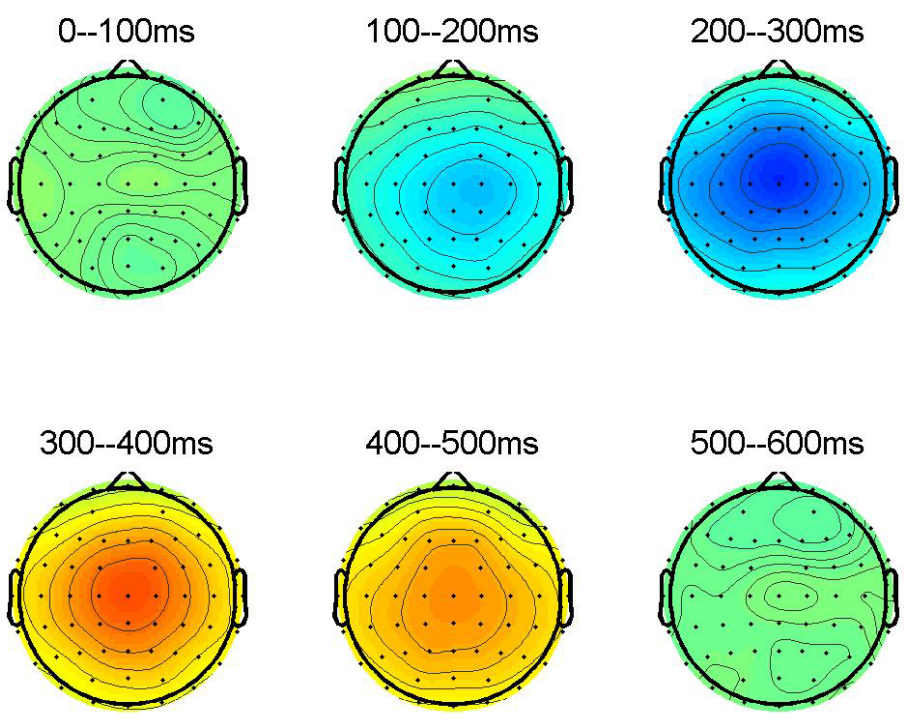
这段代码的功能是画时间系列的地形图。第一行代码是将时间轴按照从0到500ms每隔100ms画一个地形图,下面的代码是一个for循环,用来循环时间序列。代码跑完之后,会生成如下图形:
以上是本篇文章介绍的所有内容,大家可以参照样例数据跑下代码练习练习。